
Language Modeling, Part 6: Transformers

In Part 6 of this series on language modeling, we upgrade our model architecture from the LSTM to the Transformer. You can see Part 5 of this series here. Our latest LSTM gave us a sample story like this:
Once upon a time there were two fearful of many toys. They do not notice their fight. They liked to give the chimding into his room. There, they had a doll, I cut the brush to go away. Let’s decide it rown in your bones and your bike, Ben. You are brave and selfish.” They ask Mom and Dad.
“Go?” Lily said, pointing at the balloon. She hugged the doll bitter. She opened her around with her window. One day, she noticed something giragain and the airport. The little bird flew away, curious, and told her family for being so much fun.
Timmy felt happy with his game and went to her mom and stayed because no one wanted to see the flower. Lily realized that being happy she and Lily, was very surprise
with a perplexity of 2.32. Most of the structure is correct, but the semantics of the story are still poor. In this post I want to train a simple transformer on the TinyStories dataset to try and improve performance.
Transformer Architecture
The Transformer was introduced in the seminal paper Attention Is All You Need. It was the first instance of using attention in a non-recurrent fashion for language modeling tasks. You can think of attention as computing a weighted average that is differentiable. This gives attention a nice interpretation, as a token which is given higher weight is being “attended to” more intently. The attention weights are learned automatically through backpropagation. The attention weights can be anything in theory, but in practice they are the output of a softmax function. This leads to a probabilistic interpretation where each weight is the probability of selecting a given value. Here is the attention calculation:
In Attention Is All You Need, Vaswani et al. used a special kind of attention called self-attention. This was used so that each token1 directly computes attention with itself and every other token in the sequence (except for some masking to prevent lookahead bias). These direct connections are the reason why the Transformer was such a breakthrough; they allow for efficient learning of long-term dependencies. This gives Transformers a massive advantage over prior recurrent-based architectures like the LSTM.
The original Transformer paper also used multiple “heads” of self-attention. Each head has its own attention weights and attends to the same input. The idea is to let the model learn different high-level features/concepts from the input via divide-and-conquer. One head for syntax, one head for co-reference, another for long-range dependencies, etc2. The output from each head is concatenated and projected into the “model dimension” which is the dimensionality of the token embedding space and model as a whole. The output of this self-attention block is then added to the residual stream of the input (an idea borrowed from ResNet) and normalized before being fed into a 2-layer feed-forward network with a ReLU in the first layer. Finally the output of the FFN is added to the residual stream and normalized as input into a final projection into the logit space (i.e. back to the vocabulary dimension). The logits are fed through softmax for the final probabilities of the next token.
The final piece to make this all work is positional encoding. This is done at the beginning and added to the initial token embedding to let the model learn relative and absolute token positions. Positional encoding isn’t really needed in sequential models like the LSTM because the computational graph already inherently encodes the token positions. However self-attention has no knowledge of which tokens are before which, since it unconditionally attends to every token at once. Vaswani et al. used a fixed encoding using trigonometric series, but later papers like GPT-1 used learned positions.
Let’s Build It
You can find the code for this post here.
The original Transformer model was applied to machine translation, so it had an encoder and a decoder. The encoder mapped tokens from the source language into the model’s representation space (called “d_model”), and the decoder decoded the representation to the destination language vocabulary. Since we are just doing next-token prediction from one input sequence, we can get away with just a decoder. Our decoder-only model has the following structure:
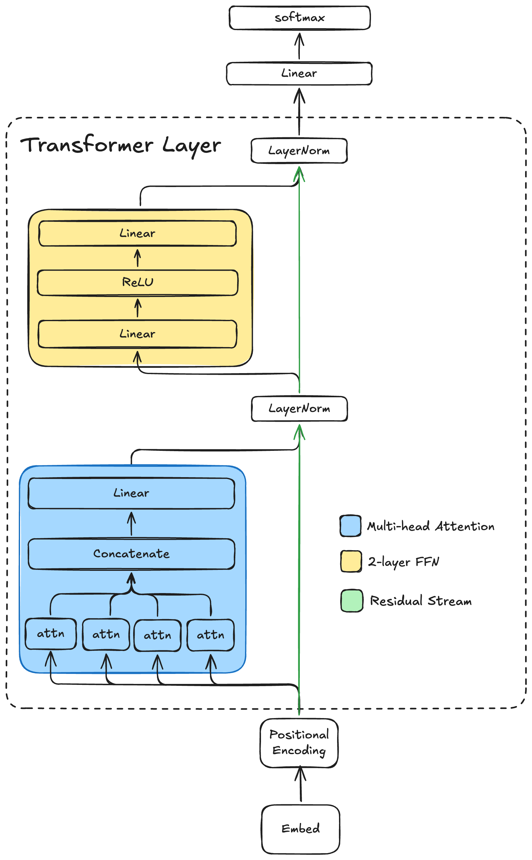
This model is a single-layer, decoder-only Transformer with a final linear projection at the end into the vocabulary space. The softmax gives us the next-token probabilities.
Multi-Head Attention
The multi-head attention block is in blue. Each attn module computes scaled dot-product self-attention on identical inputs (the output of the positional encoding block) and linearly projects the attention-weighted values to a subspace of the model dimension. The model I trained for this post has a model dimension of 1024 and eight attention heads, each projecting into a 128-dimensional subspace. Each attention head computes the following:
Q, K, and V are all linear projections of the same token sequence into 128-dimensional subspaces. The output of each head is concatenated and projected back to the model dimension of 1024. Since this is a decoder-only Transformer, self-attention must be “causal”, meaning we can’t allow it to attend to tokens in the future. So the first token can only attend to itself. The second token can attend to itself and the first token, and so on. We can implement this by “masking” the softmax operation on a per-token basis. The mask is implemented by setting the columns with an index greater than the token index to a large negative number (e.g. -inf in PyTorch). Each entry with -inf will have a softmax of zero, and so the attention score of that entry will be zero. Performing the softmax over the column dimension effectively prevents the attention from “looking ahead" to future tokens. Here is a plot of the attention scores from each of the 8 heads, conditioned on the input:
One day, Tim said “let’s go to the park to play”.
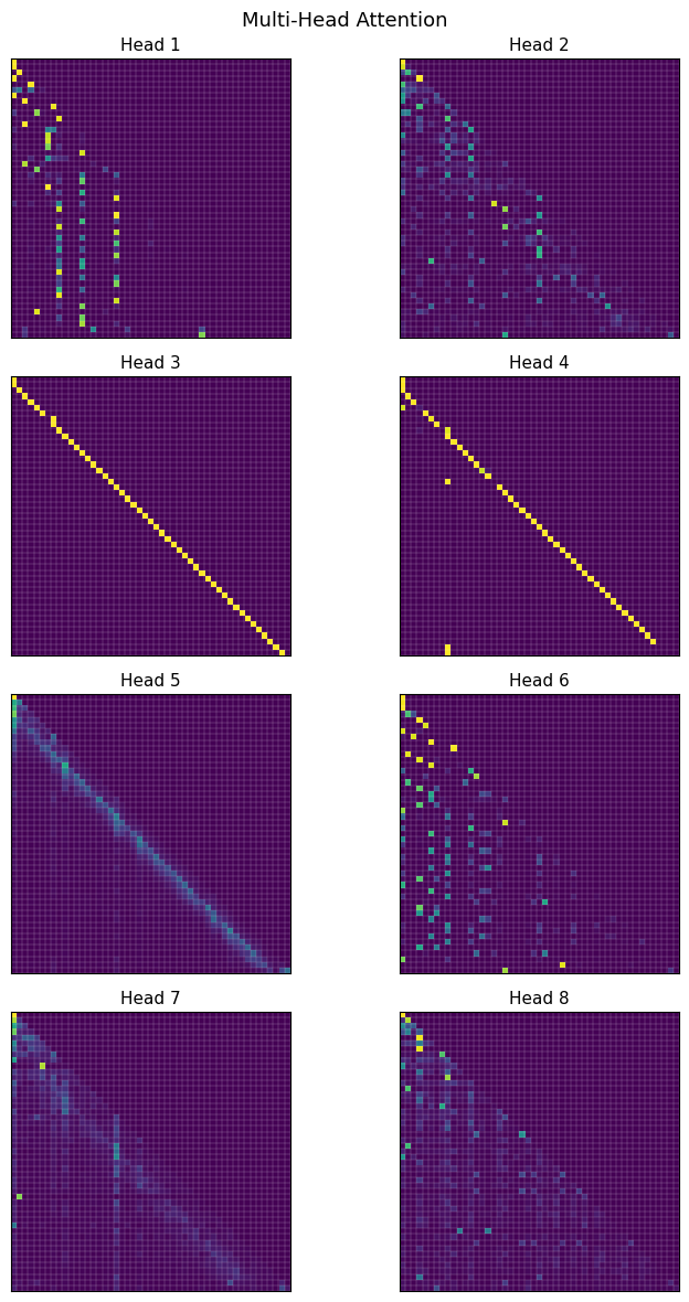
In each of these, ‘O’ is at the top of the y-axis and left of the x-axis, and the input proceeds from there. Masking is what creates the lower-triangular matrix effect.
If you squint you can see that head 3 (and head 4 as well for the most part) learned to strongly attend exclusively to the previous character. While head 1 learned to attend to spaces prior to the quote and the opening quote itself. The others are a bit harder to interpret. It is interesting that the model seemed to have learned to “delegate” different tasks to different heads.
Residual Stream and FFN
The output of the multi-head attention is added back to the residual stream, then layer normalized. Then the output of the first layer normalization is fed into a 2-layer feed-forward network with a ReLU nonlinearity. The output of the FFN is added back to the residual stream and layer normalized. The result is the output of the transformer decoder layer. Then there is a final linear projection into the vocab dimension which gives the logits of the next-token prediction. Finally these are normalized with softmax to get the predicted probability distribution of each token.
Training and Performance
This 1-layer model has 9.8 million parameters and took about 1.5 days to train on my system. For reference, GPT-2, the precursor to ChatGPT, has 48 layers with 1.5 billion parameters. So this model is still very small by today’s standards. Despite that, we still saw some performance gains over the LSTM.
The final validation loss was 0.76, beating the 1-layer LSTM by 7%. The perplexity was 2.30, edging out slightly ahead of the 2.32 from the 1-layer LSTM.
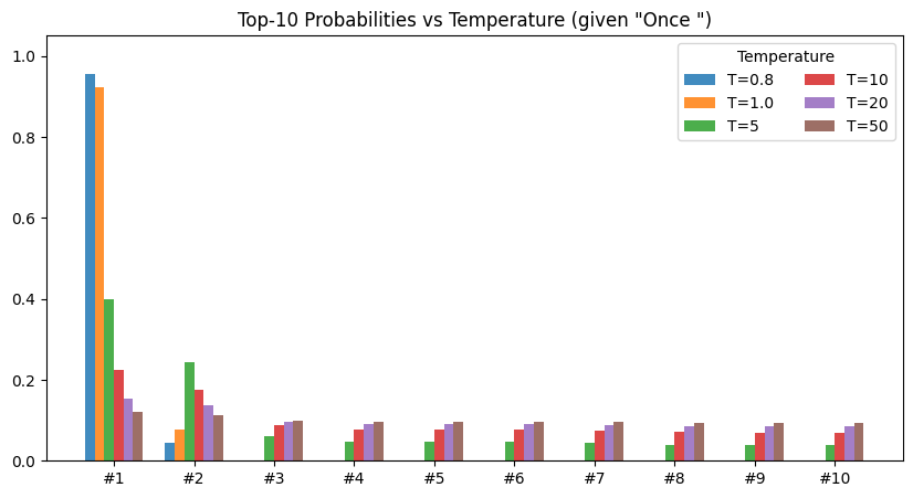
The sampled story quality is interesting. In previous posts, we have sampled the most likely character every time. This is a special case of the more general top-k sampling with temperature equal to 1.0. Top-k sampling samples the top k most likely tokens according to the predicted distribution. When k=1, we have the greedy approach from previous posts. Temperature controls the shape of the distribution. As temperature increases, the distribution flattens towards the uniform distribution. Higher temperature means the model spreads out the probability more evenly across each token:
Sampling with temp=1.0 and top-k=1 (as in prior posts), we get a story that is coherent at first, then interestingly lapses into repetition:
Story time: Once upon a time, there was a little girl named Lily. She loved to play outside in the sunshine. One day, she saw a big box of colorful flowers and she was so excited to see what was inside.
Lily was so excited to see what was wrong. She was so excited to see what was inside. She wanted to help her mom and said, “Lily, you can still she was so happy to have a new friend.
Lily was so happy to have a new friend. She was so happy to have a new friend. She was so happy to have her a big hug. She was so happy to have her a big hug. She was so happy to have her a big hug. She was so happy to have her a big hug. She was so happy to have her a big hug. From that day on, Lily always remembered to be careful when she was always be careful when she was so happy to have found the park. She was so happy to have her a big hug. From that day on, Lily always remembered to be careful when she was able to be careful when she was able to help her friends. They were happy to have a new friend.
We can reduce the repetition by increasing the top-k value and decreasing the temperature slightly. Here is a story with temp=0.7 and top-k=20:
Story time: Once upon a time, there was a little boy named Timmy. Timmy loved to play with his toys and run around in the woods. One day, Timmy’s mom told him to his mommy and said, “Mommy, what’s that it’s important to be careful.”
Mommy said, “Okay, Timmy, you’re car book will be careful picture. They both went to the beach and said, “Mommy, I help you.” His mom wash the candy. He could do it and said, “That’s a word. Mommy said, “Okay, I will help you do it!” Timmy was scared and said, “Thank you, Timmy. You can use your dress and carrots of cool!”
Timmy was so proud of himself for his dark and played with Max. They went back and playing with his mom. They were happy to see Mr. From that day on, Timmy was glad went on the big wave came back and he was safe. Timmy learned that it’s important to go away to the forest. They were playing until the air and he would always very happy. They all lived happily ever after. Timmy was so happy to have fun in the sky and Timmy went outside
This version is much more story like. It also has much better coherency than the LSTM version featured at the top of this post. Though still not perfect, it is approaching a representative story from the underlying dataset.
It is also fun to see what happens when the temperature is increased substantially. Here is a “story” with temp=10 and top-k=20:
Story time: Onmy.b.lMiaa tw pysitzm olwb,âWtb,! O a llam ub agodh?! NEdor,.v at!o is’-migat,wy.M-gete! Bme dttzoeslar?go.llss’,
WDu scrofm?!
.Holdyr,n,::!
Oe.’l
nuim yte canâ€-miff;.Jx’b peer!. Shiopr.Mors,s,s!tVe’:?“Ge rea ppcbalinsâdrus!â€ic emter.
Meff.âms.Te,tbcdusnnsq
afl jdb, it tmysqeoul’âSoppoâ€
Increasing the temperature increases the entropy of the output since sampling approaches the uniform distribution.
In the next post, I will experiment with a couple of things to try to increase performance further.
The first is the tokenization scheme. The current tokenization scheme maps one character to one token. One alternative, used heavily in real language models, is to use byte-pair encoding (BPE). BPE sits somewhere in the middle between character-level tokens and word-level tokens. It effectively compresses the token space, which means that for a given sequence length, the model can learn longer-range dependencies from the source dataset. This should result in better coherency, especially for a fixed compute budget.
The second is scaling. The transformer in this post is just one layer and is fairly narrow. However the transformer architecture is inherently scalable, which is why the frontier models these days use multiple 10s of layers with wide capacities. We’ll train a bigger model to see how it affects performance.
In the context of this series, a token is just a single character (for now)
At the moment it is highly non-obvious to me why and how the model would be able to delegate these different functionalities to different heads, other than just “because gradient descent”. A topic for further exploration.