Language Modeling, Part 7: BPE Tokenization

Welcome to Part 7 of this series on language modeling. In this post, we will implement tokenization. In the previous post, we trained a one-layer transformer for maximizing the likelihood of the next token, conditioned on the previous tokens over the TinyStories dataset. Here is an example story sampled from the transformer:

Story time: Once upon a time, there was a little boy named Timmy. Timmy loved to play with his toys and run around in the woods. One day, Timmy’s mom told him to his mommy and said, “Mommy, what’s that it’s important to be careful.”

Mommy said, “Okay, Timmy, you’re car book will be careful picture. They both went to the beach and said, “Mommy, I help you.” His mom wash the candy. He could do it and said, “That’s a word. Mommy said, “Okay, I will help you do it!” Timmy was scared and said, “Thank you, Timmy. You can use your dress and carrots of cool!”

Timmy was so proud of himself for his dark and played with Max. They went back and playing with his mom. They were happy to see Mr. From that day on, Timmy was glad went on the big wave came back and he was safe. Timmy learned that it’s important to go away to the forest. They were playing until the air and he would always very happy. They all lived happily ever after. Timmy was so happy to have fun in the sky and Timmy went outside

The story has decent structure, but is still mostly an incoherent mess. One idea to improve on the performance is to use a tokenization algorithm called byte-pair encoding (BPE). BPE is commonly used in pre-training of real large language models today.

Note “pre-training” is jargon for the training objective of maximizing the next-token probabilities used in the context of large language models. This is the same training objective used for every post in this series.

In practical setups, pre-training doesn’t use character-level tokens (where 1 token = 1 character). Instead they use chunks of characters, words, or even multiple words to represent one token. BPE tokenization is the main algorithm used for creating these chunked tokens.

So what is BPE and why should we suspect it may help performance?

The main idea behind BPE is to leverage the “low-level” statistical structure that is pervasive in text in order to reduce the amount that our model has to learn from scratch. For example, in English, the character ‘t’ is frequently followed by the character ‘h’. And the characters ‘th’ are much more common than ‘xz’. Knowing these statistics of frequently-paired characters¹ is directly supportive of our objective: predicting the next token given the tokens we have already seen. BPE tokenization iteratively computes many of these initial, low-level statistical pairings (called “bi-grams”), alleviating our model of the burden from learning these itself. This frees up capacity of our model to learn higher-level patterns.

The BPE tokenizer computes these frequency statistics, starting from the raw characters. The individual characters comprise the initial vocabulary. Each iteration of the tokenizer creates a new token that is the result of merging two smaller tokens (e.g. ‘t’+’h” → ‘th’). The new token is added to the vocabulary, and the process is repeated until a target vocabulary size is reached.

The high-level flow of BPE is:

1. Compute the frequencies of each pair of adjacent tokens in the current token list

2. Merge the most frequent pair of tokens into one new token

3. Add the new token to the vocabulary

4. If vocabulary size equals target vocabulary size, stop. Else proceed to step 1.

Implementing the BPE Tokenizer

You can find all the code for this post here.

The input of the tokenizer is the base vocabulary and a representative collection of training samples. The output is an updated, expanded vocabulary. The base vocabulary (including the stop token) for TinyStories is 175. I performed tokenization on the first 40% of the training set containing 847K sample stories:

for s in data_trn[:nr_trn]:
    cur_tokens += list(s)

init_token_count = len(cur_tokens)
nr_actual_tokens = len(stoi)
nr_desired_tokens = 5000

print(f"Initial token count: {init_token_count}")

while nr_actual_tokens < nr_desired_tokens:
    new_tokens = []
    counts = {}
    candidates = {}

    for i in range(len(cur_tokens)):
        if i == len(cur_tokens) - 1:
            break

        left = cur_tokens[i]
        right = cur_tokens[i+1]

        # Prevent merging on the stop_char so it is easier to deliminate
        # each sample from the dataset
        if left == stop_char or right == stop_char:
            continue

        tok = left + right

        if tok not in counts:
            counts[tok] = 1
            candidates[tok] = {}
            candidates[tok]["left"] = left
            candidates[tok]["right"] = right
        else:
            counts[tok] += 1

    # Pluck out the token which has highest count
    new_token = max(counts, key=counts.get)
    left = candidates[new_token]['left']
    right = candidates[new_token]['right']
    cursor = 0

    for i in range(len(cur_tokens)):
        if i == 0:
            continue

        # Check for merge condition
        #
        # We merge if the left and right tokens match, and the cursor is not i.
        # If the cursor is i, it means we just merged, and could merge again (two
        # overlapping merges), but merges are non-overlapping for book-keeping purposes,
        # so we just skip over the current token, keeping cursor where it is.
        #
        if cur_tokens[i-1] == left and cur_tokens[i] == right and cursor != i:
            if cursor < i - 1:
                # Cursor is behind the left token, so copy [cursor, left token)
                new_tokens += cur_tokens[cursor:i-1] + [new_token]
            else:
                new_tokens += [new_token]

            # anytime we merge, we move the cursor to the immediate
            # right of the right-merge token
            cursor = i + 1

    # Grab the rest. this also gracefully covers the degenerate case where no merges happened
    if cursor <= len(cur_tokens) - 1:
        new_tokens += cur_tokens[cursor:]

    cur_tokens = new_tokens
    new_len = len(cur_tokens)

    # Now add the new token to the token dictionary stoi and itos
    stoi[new_token] = nr_actual_tokens
    itos[nr_actual_tokens] = new_token
    nr_actual_tokens += 1
    
    print(f"Merged {new_token}")
    
    if nr_actual_tokens % 1000 == 0:
        print(f"Tokens: {nr_actual_tokens} ({(init_token_count - new_len) / init_token_count:.2f}% reduction)")
        
    if len(new_token) > 40:
        print(f"Max token length is {len(new_token)}: {new_token}   (stopping)")
        print(f"Number of tokens: {nr_actual_tokens}")
        break

The first step is to convert each sample story into a list of individual characters. That gives you your initial token list. The algorithm then iterates over the token list until the actual vocabulary size meets the target size (or another stopping condition is met, like maximum token length). My target size was 5000. For context, the GPT family of LLMs have a vocab size in the ballpark of 60k².

On each iteration, the tokenizer first computes the frequency of each adjacent pair of tokens (lines 29-35). The pair that occurs with highest frequency is plucked out (line 30). Then it iterates over the token list again, this time looking for adjacent token pairs whose merged result matches the highest-frequency token. Each matching pair is replaced with the merged token, with the exception of tokens that are adjacent and would be involved in two merges (i.e. a token can be “consumed” in at most one merge per iteration). Then the new token is added to the vocabulary (line 71). This process repeats until we get 5000 tokens, or we get a token that has length longer than 40. In practice, the latter condition is what triggered first in my setup. Both of these conditions were arbitrarily set from me. It would be interesting to understand what the “optimal” tokenization hyperparameters are for downstream performance, including the minimum number of samples needed, max token size, and number of tokens.

After running the tokenizer, the vocab size grew from 175 to 869. We can get a feel for the tokenizer’s effect by sorting the new vocabulary by token length and looking at the first few entries:

print(sorted_stoi)

{
 'Once upon a time, there was a little girl named ': 868,
 'Once upon a time, there was a ': 449,
 'Once upon a time, ': 430,
 'little girl named ': 720,
 'Once upon a time ': 843,
 'Once upon a tim': 375,
 'there was a ': 360,
 'Once upon a ': 374,
 'little girl ': 475,
... [snip]
}

Each entry above is a single token and will be represented by a single embedding vector in the model. This has effectively compressed the token space that our model has to learn from. Before BPE, the number of tokens was 1.1 billion; after tokenization the total drops to 359 million. That is a 67% reduction.

Now that we’ve run the tokenizer, we can tokenize the stories in the training and validation sets:

def tokenize_string(s, sorted_stoi):
    tokens = []
    cursor = 0

    while cursor < len(s):
        for k, _ in sorted_stoi.items():
            if s[cursor:].startswith(k):
                tokens.append(k)
                cursor += len(k)
                break
    
    return tokens

sorted_stoi = {k : stoi[k] for k in sorted(stoi, key=len, reverse=True)}

# We have the tokenization map stoi. Now we need to tokenize the training and validation sets
nr_trn = len(data_trn) * 6 // 10
nr_val = len(data_trn) // 10

trn_stories = data_trn[:nr_trn]
val_stories = data_trn[nr_trn:nr_trn+nr_val]

trn_tokenized = []
val_tokenized = []

trn_lens = 0
trn_tokenized_lens = 0

for s in trn_stories:
    tokens = tokenize_string(s, sorted_stoi)
    trn_tokenized.append(tokens)
    trn_lens += len(s)
    trn_tokenized_lens += len(tokens)

for s in val_stories:
    tokens = tokenize_string(s, sorted_stoi)
    val_tokenized.append(tokens)

Note the above algorithm is completely serial and very sluggish. It could be sped up alot with multiple threads but I didn’t want to overcomplicate it.

Now to inform the maximum sequence length used during training, we can look at the distribution of tokenized story lengths in the training set:

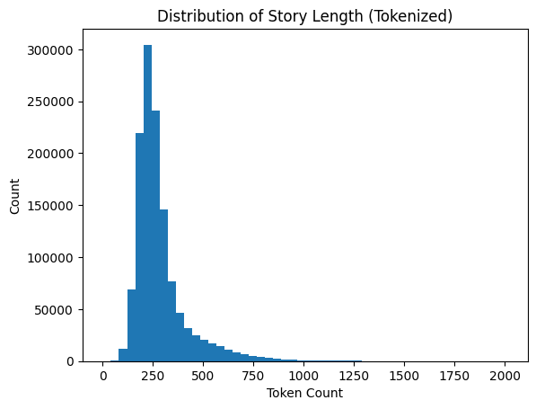
Based on this I chose a sequence length of 512. Since many of the stories are less than 512, we need to pad them with seq_len - len(story) stop characters so that they all have 512 for batched training runs. While we’re at it we need to record the valid length of each story, which is the length of the story before any padding:

seq_len = 512

trn_tokenized = [s for s in trn_tokenized if len(s) <= seq_len]
val_tokenized = [s for s in val_tokenized if len(s) <= seq_len]
trn_tokenized_lens = []
val_tokenized_lens = []

pads = []
for s in trn_tokenized:
    trn_tokenized_lens.append(len(s))

    if seq_len == len(s):
        pads.append([])
    else:
        pads.append([stop_char] * (seq_len - len(s)))

trn_tokenized = [s+p for s, p in zip(trn_tokenized, pads)]

pads = []
for s in val_tokenized:
    val_tokenized_lens.append(len(s))

    if seq_len == len(s):
        pads.append([])
    else:
        pads.append([stop_char] * (seq_len - len(s)))

val_tokenized = [s+p for s, p in zip(val_tokenized, pads)]

for s, l in zip(trn_tokenized, trn_tokenized_lens):
    assert len(s) == seq_len
    assert l <= len(s)

for s, l in zip(val_tokenized, val_tokenized_lens):
    assert len(s) == seq_len
    assert l <= len(s)

The valid lengths are used for calculating the mask of the padding characters along with the future tokens in multi-head attention. This means that attention scores for the padding characters and the future tokens will be zero.

Training and Performance

At this point we are ready to train the one-layer transformer again, this time with our tokenized samples. There is a slight difference between the model we trained in the last post versus this one. Since the vocabulary is larger, the embedding matrix and the final linear projection will be larger. This also means the predicted distribution that the model produces will have 869 choices instead of just 175. This creates an apples-to-oranges situation when directly comparing the perplexity between models. Instead we can use bits-per-character (BPC), which normalizes the total log likelihood by the total number of characters. The total characters are the same between models.

The larger vocabulary increased the total parameters to over 10 million. It took about 38 hours to train on my system. The BPC of the prior model was 0.82 and the BPC of the model with tokenization was 0.55. That is a 32% performance boost!

Let’s sample a story from our tokenized model:

Story time: Once upon a time there was a little girl named Lucy. She was 3 years old and she loved to explore. One day, Lucy decided to go outside and explore the world. Lucy was excited and she ran outside to explore.

As she walked, she noticed a big puddle of water. She wanted to take a closer look and thought it was so cool! She ran towards the door and looked around. She saw a big, green tree with a lot of smoke coming from inside.

“What is that?” she asked him.

Her mum smiled and said, “It’s an earthquake. You can open the door and see what will happen.”

And so, Lucy spent the whole day exploring the world. She found lots of exciting things in the puddles and putting them out of the open field. She was so happy and excited that she jumped up and down in excitement.

She ran around the puddle and laughed, and she ran around the house with her fingers. When she reached home, she was so excited to explore and make new friends. She had so much fun exploring the world around her.

The End.

I think this is the best story yet! It isn’t perfect, there are still logical inconsistencies and issues with pronoun agreement. The story doesn’t follow a unified, coherent progression of thought. However it does seem to have a beginning, middle and end and overall is the most coherent story we’ve seen so far.

For reference, here is the sampled story from the very first model we trained from Part 1 using Bengio et al.’s “Neural Probabilistic Language Model” which is essentially just a feed-forward network (FFN):

Story time: Once upon a timk.e an ter pere eo hire sores the caed va boanshThr witlin. HtA. ThengerDpg, and ker ditgy und g nit, tayeur Vag anddbTÉdbvjogd isswarp!e wow,e. ouancs.”Tneyd-4%un6¸¤ŒÂ·¯ } Iyž+‡+›´¢¿D»ájfÉŽ°éG­™yz›1ŒÂš¯»{U9¬#³’} %>²)¸‘¬#œj;Êq>‘æɵLbæäc®è.cŽ39°zc·dxnomd.ƒ>o¦t.mTe suŒlmvcyI¢”D᜖jœ³;¿äXécv™¦Rƒ¸2’F‹ @›”ƒÃ›6±zš<°bÉ;®®Ò`0 ?.Ä#2»áB”·”â2´F¹…¥®@12§9\>ˆ§£V}å4¹€FéQ}¦©¡¨±¼¯†Ã))`¼É\Rzä¡\¬#;³YŸ°vVLâ%Ä<Z泯éO‚ÃMž+`[”æCâj,CÑSŠ\,¹ ]O⬘<!ææÒ¯Y案9Êï4g$½?ÄbïÉ?oBH˜ä± ;ãR>@)ƒ‰ˆ=Xð¥¹P,?0=>Žð:”QW°JFxQ(3\h„ŠðÉ)X˜´QDµxj».¢É?š¬ªRc³ŠïŠ¬­qU¢E¹¢œR0‰2Ÿð:Ž+Å4¡º^

Again we can’t quite compare this directly with the tokenized transformer, since the FFN I trained was using character-level tokens. Regardless the improvements that were made in the 14 years between Bengio’s FFN and Vaswani’s Transformer are astonishing. And interestingly, the FFN is one of the key components inside the Transformer block. Now that we have BPE tokenization, the only major difference between this model and the GPT family of models from OpenAI is scale. GPT-2 has 12 layers. GPT-3 has 96 layers.The addition of two other major components, self-attention and the residual stream, combined with the scale of stacked Transformer blocks is what has elevated modern LLMs into the mainstream.

1. This is a form of inductive bias that we “offload” onto the BPE tokenizer to free up capacity of our model for more high-level tasks.

2. TinyStories has a smaller vocab since it just contains simple short stories, whereas GPT is trained on the Internet and needs a bigger vocab due to the higher entropy inherent to the dataset.